
On The Origin of Time-Sharing Computers, Round-Robin Algorithms, and Cloud Computing
Introduction
Recently I began writing a post on ways to automate python scripts passively.1 For the purpose of the post I chose cron, an operating system utility that is run as a daemon—a program that runs passively in the background of a computer. If cron and daemon both seem etymologically Greek to you, they did to me as well. While researching whether this was true (it probably is), I fell down an interdisciplinary rabbit-hole of computer science history. What I discovered and have since written about below is a more complete history than I've been able to find about time-sharing computing and the function of the round-robin algorithm. In future a post, I plan on writing more about the economics of cloud computing.
Early Innovations
In the early 1960s, the Advanced Research Projects Agency (ARPA)2 was investing in different projects that could be used to fight the Soviets. The agency, only a few years old, had been founded just four months after Sputnik's October 1957 launch. Its express mission was to maintain the US's technological (military) superiority over other nations. With an initial budget of $400 million dollars (about $3.7 billion in 2020 dollars), the agency had few limits.
One such project that received ARPA funding was the politically named Project MAC (Mathematics and Computation) out of MIT. Established by computer scientists Robert Fano and Fernando José Corbató in 1963, by calling the endeavor Project MAC Fano and Corbató were able to attract researchers from existing labs without anyone's loyalties (or funding) being questioned.

Project MAC had multiple objectives, but its main focus was Corbató's previous work on time-sharing systems. Though many strides in computer hardware and software had been made over the previous decade—the invention of the compiler3, the use of the transistor computer4, and the creation of FORTRAN, LISP, and COBOL5—there were still struggles. Despite all the progress computing had made in the previous decade, compute-time—actually using the computer—remained cumbersome.
For efficiency, batch-processing was used for computation: decks of punch cards featuring multiple programs were encoded onto magnetic tape and fed by an operator into a central computer for iterative processing. But while a computer read the program, its central processor remained idle: a waste of precious compute-time. And, if errors occurred in a program itself, then hours had to be taken to debug it by hand.6 Even when the code was actually fixed, a program still had to be rewritten onto a new magnetic strip and subsequently rescheduled by an operator for computation. So frustrating was this process that in 1967 students at Stanford took to producing a humorous (if dated) short film about the matter.
Sharing Time: Round Robin and Multilevel Scheduling
In recognizing how burdensome compute times were, Corbató laid out his plans for "the improvement of man-machine interaction by a process called time-sharing" in a 1962 paper submitted to the International Federation of Information Processing (IFIP). Like many computer science-related projects of the time, time-sharing was a concept that emerged from military operations. In the late 1950s, the North American Air Defense Command (later known as NORAD) had begun operating a first-of-its-kind network of IBM-manufactured computers connected to near real-time radar data. The Semi-Automatic Ground Environment (SAGE) air-defense system was unique, not only its capacity to detect Soviet missiles, but also in its ability to programmatically loop through its systems in as little as 2.5 seconds. John McCarthy, a computer scientist from MIT who had seen a prototype of SAGE, was inspired enough to conceptualize a similarly fast system to be used by multiple programmers at once. In a memo sent out to the MIT community, McCarthy outlined how such a shared-system would work. Corbató, picking up the mantle, aimed to make tangible such a system. But, as so often happens with the popular usage of terms in computer science, even trying to communicate what Corbató meant by time-sharing became confusing.7 Corabtó explained the multiple meanings of time-sharing in his 1962 paper:
One can mean using different parts of the hardware at the same time for different tasks, or one can mean several persons making use of the computer at the same time. The first meaning, often called multiprogramming, is oriented towards hardware efficiency in the sense of attempting to attain complete utilization of all components. The second meaning of time-sharing, which is meant here, is primarily concerned with the efficiency of persons trying to use a computer.
Unlike the SAGE system which was a feat of multiprogramming, Corbató aimed to make real the latter definition with Project MAC. And, with the wind at their back and ARPA funding in their pockets, Corbató and his colleagues were able to succeed in this, compiling new commercially viable hardware and software systems such that multiple individuals could seamlesly submit code to a central processor. Users would access a mainframe computer remotely via their very own typewriter console. Constantly running in the background would be a multilevel queuing routine which would schedule program calls by priority: determining whether a submitted program was a foreground process or a background process. Once queued, these programs would then be operated by a Round-Robin algorithm8 that ran queued programs for set slices of time, in this case approximately .2 seconds, which Corbató estimated was the speed of human reactivity.
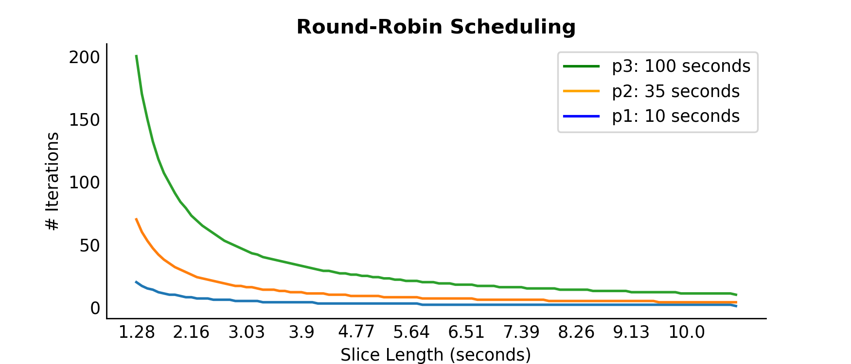
An example of the Round-Robin algorithm can be seen in the first chart below. Given a program  that takes
  seconds to run, each program is limited to run for a length of time
  . If
. If  then after seconds is paused, sent back to the queue with time
  left, and set to continue running once it reaches the head of the queue again. This process continues until all programs in the queue have fully completed. The benefits of the Round-Robin algorithm, and why it was used with the advent of time-sharing computers, was the priority response time took in computing, where response time is the time difference between when a programmer enters a program into a queue and when it begins to first run. Recall that programmers wanted to start their programs as soon as possible in order to reduce CPU idle time. As can be seen, as the slice of time decreases to the left of the x-axis, the number of iterations—or loops through the queue—increase exponentially on the y-axis. As the length of the time slice increases to the right of the x-axis the number of iterations decrease on the y-axis. This is the case for all three different programs of length 10, 35, and 100 seconds.

Expand for Code
# Load Libraries

from timeit import default_timer as timer
from collections import defaultdict
from collections import deque
from typing import Dict
from typing import List
import pandas as pd
import numpy as np

# Plotting
from matplotlib.lines import Line2D
import matplotlib.pyplot as plt
import matplotlib as mpl

mpl.rcParams['figure.dpi'] = 250
#
# Round Robin Simulation
def round_robin_scheduling_sim(p1: List[int], p2: List[int], p3: List[int], time_slice: List[float]) -> Dict[str, List[int]]:
"""
Given three programs (p), where each program has a different program length (t),
quantize or time-slice some fixed amount (q) to simulate a round-robin scheduler.
---------------------
Params:
p1,p2,p3: arrays of form [program, program_length, iteration count, response time]

time_slice: length of to run program before continuing in queue
---------
Returns:

program_dictionary: dictionary of program keys and number of iterations given time-slices
"""

        # create a list to collect results
        time_slice_results = []

        # for each time slice (q), loop through the round-robin scheduler
        for time_slice in time_slice_list:

                # record time program entered in queue...
                parent_arrival_time = timer()

                # ...into response time position in each list
                p1[3] += parent_arrival_time
                p2[3] += parent_arrival_time
                p3[3] += parent_arrival_time

                # create tuple of structure: program, program_length, iteration count, response time
                program_tuple = [p1, p2, p3]

                # program tuple enters queue
                program_queue = deque(program_tuple)

                # create list to collect short-term results
                result_list = []

                # begin round-robin scheduler: loop while a program is in queue
                while len(program_queue) != 0:

                        # access program and unpack tuple
                        program, program_length, iteration, arrival_time = program_queue.popleft()

                        # if response time has not been calculated, calculate it
                        if parent_arrival_time == arrival_time:
                                # response time: first-run - arrival time
                                arrival_time = timer() - arrival_time

                        # run program for length of time-slice, and record results
                        program_length = program_length - time_slice

                        # if program still has positive value, it is incomplete
                        if program_length > 0:
                                # record that an iteration has been run
                                iteration += 1
                                # place unfinished program back into end of queue
                                program_queue.append([program, program_length, iteration, arrival_time])

                        # if program is zero or negative, it has completed its run-time
                        else:
                                # record last iteration
                                iteration += 1
                                # record which program has finished, and iteration count
                                result_list.append((program, iteration, arrival_time))

                #after all programs have left queue, record results
                time_slice_results.append(result_list)

                # reset iteration count, arrival time for next run
                p1[2], p1[3] = (0,0)
                p2[2], p2[3] = (0,0)
                p3[2], p3[3] = (0,0)

        # unpack results into single list of tuples
        time_slice_results_single_list = [x for y in time_slice_results for x in y]

        # organize single list into dictionary
        program_dictionary = defaultdict(list)
        for program, iteration, arrival_time in time_slice_results_single_list:
                program_dictionary[program].append([iteration, arrival_time])

        # return dictionary of results
        return program_dictionary

def response_time_simulation(x: int)->plt.Figure:
"""
Loop x amount of times through round-robin scheduler,
track response times, and plot average of all x response times,
where average response times:

average response time = sigma {i,n} first-run_i - queue-time_i / n
for each program p
----------------------
Parameters:

x: number of simulations to run
----------------------
Returns:

plt.Figure: plot of simulations
"""

# generate 100 different slices (q) between 10 and .5 seconds
time_slice_list = [round(q,2) for q in np.linspace(10, .5, num = 110)]
average_response_list = []
for i in range(1000):
        program_dictionary = round_robin_scheduling_sim(p1=['p1',10,0,0],
                                                                                                p2=['p2',35,0,0],
                                                                                                p3=['p3',100,0,0],
                                                                                                time_slice=time_slice_list)

        average_response = [(x[1] + y[1] + z[1])/3 for x,y,z in zip(program_dictionary['p1'],
                                                                                                                                program_dictionary['p2'],
                                                                                                                                program_dictionary['p3'])]
        average_response_list.append(average_response)

fig, ax = plt.subplots(figsize = [7,3])
ax.plot([x[0] for x in program_dictionary['p1']][::-1], label = 'Program 1')
ax.plot([x[0] for x in program_dictionary['p2']][::-1], label = 'Program 2')
ax.plot([x[0] for x in program_dictionary['p3']][::-1], label = 'Program 3')

custom_lines = [Line2D([0], [0], color='green'),
                                Line2D([0], [0], color='orange'),
                                Line2D([0], [0], color='blue')]

ax.legend(custom_lines, ['p3: 100 seconds',
                                                'p2: 35 seconds',
                                                'p1: 10 seconds',])

plt.xticks(np.arange(0, 110, 10), labels=time_slice_list[::10][::-1])

# remove tick marks
ax.xaxis.set_tick_params(size=0)
ax.yaxis.set_tick_params(size=0)

# change the color of the top and right spines to opaque gray
ax.spines['right'].set_visible(False)
ax.spines['top'].set_visible(False)

# set labels
ax.set_xlabel("Slice Length (seconds)")
ax.set_ylabel("# Iterations")

# alter axis labels
xlab = ax.xaxis.get_label()
ylab = ax.yaxis.get_label()

xlab.set_size(10)
ylab.set_size(10)

# title
ax.set_title("Round-Robin Scheduling")
ttl = ax.title
ttl.set_weight('bold')

if __name__ == "__main__":
    response_time_simulation(1000)
For programmers who wanted their programs running as soon as possible, the usefulness of the Round-Robin scheduler can be seen in the response time chart above. Just as before, the x-axis represents the measure of different periods of time programs are run for before being paused and re-queued. The y-axis, however, now represents the average response time  of all programs: where average response time is the difference between when a program is entered into the queue
  and when it first begins to run
  . Together, the variables form the equation below:
![\[\bar{r}=\frac{\sum\limits_{i=1}^n {p_q}^i}{n}\]](https://benjaminlabaschin.com/wp-content/ql-cache/quicklatex.com-e254851dcf33f54192f8500e9a90b465_l3.png "Rendered by QuickLaTeX.com")
Notably, programs initially placed at the end of the queue will by definition have longer response times than those initially placed at the front of the queue if these programs are submitted at the same time. So, even if two progams are comparatively similar, their response times may differ. Not only that, but by using the Round-Robin algorithm with shorter time slices, submitted programs would be iterated over more frequently, as seen in the first chart. Despite this increase, time-sharing still allowed for a lower average response time for submitted programs compared to their pre-time-sharing alternatives, as seen in the second chart. Said another way, the difference between the exponential rise in average response times to the far-right of chart and the low response times to the far-left illustrates the significance of time-sharing before and after its invention.
From Time-Sharing to the Personal Computer to Cloud Computing?
Of course, the simulations shown above are simplifications. For one thing, the hardware that ran these simulations—a simple Macbook pro—is far more powerful than anything that was available at the time of Project MAC. Omitted completely has been any mention of other extraneous factors such as the cost of context switching, which can overwhelm computers if time slices are set too short. In other words, unlike the charts above, in reality there is a lower-bound on the efficiency of short-duration time slices. Finally, and as Corbató readily admitted, as more individuals used a system at once or if programs became more complex, response times would be negatively affected. Both factors that were sure to increase with time.

Diseconomies of scale and program complexity were, in part, contributing factors into why time-sharing computers did not become ubiquitous. But they were not the sole reason. As computer prices declined and processing power improved, it became more feasible for individuals to simply access their own computers, with their own CPU's, to run their programs. As the chart above indicates from William Nordhaus' illuminating 2007 paper, Two Centuries of Productivity Growth in Computing, computing power since the mid-19th century—if expanded to include manual computational power—was, per second, increasing rapidly in the 1960s.9 More specifically, by indexing manual computation to 1 computation per second (generous), the chart plots all other means of computation per second relative to that 1. By the 1960s, for example, computing power was approximately 1 million times greater than the index at 1850. In the decades to come, that computational power would only increase.
The second chart, seen below, depicts the cost of millions of computations per second, weighed by a 2006 GDP price index. Beginning in 1850, Nordhaus estimated a cost of approximately $500 per million computations by hand. By the 1960s, the cost per million computations by computer declined to  the cost of manual computation. By 2006, the computation cost of computers would decline by a factor of 7 trillion. That is to say, the best computers in 2006 were 7 trillion times less costly per million computations compared to the manual-based index.

So, computing costs became cheap, and as they cheapened, the need to share resources became less pressing and time-sharing became less commercially prominent...but not forever. As with so many great ideas, time-sharing had other applications amenable to our modern needs—needs that Corbató himself anticipated. In his 1962 IFIP paper, Corbató expounded upon the many benefits to time-sharing. Prominent in the paper was his suggestion that time-sharing had "numerous applications in business and in industry where it would be advantageous to have powerful computing facilities available at isolated locations with only the incremental capital investment of each console."
Today, despite the affordability of conducting millions of computations per second on a personal computer, there are still computationally intensive algorithms and Big Data operations that businesses want to engage in. In order to do so, it can make sense for these businesses to engage in cloud-computing, which, in essence, is the rental of severs of virtual machines at isolated data warehouses for the processing of these computationally intensive operations. Although not 1-to-1, cloud computing very much relies on the precedent set by Corbató's time-sharing work, and in particular the idea that multiple users could queue programs at will to a computer for processing.
We have Corbató's work on time-sharing to thank for the ability to process for much of the cloud in data science today—espcially when it comes to processing our work in the cloud on clusters of computers. As someone who was trained in economics, rather than computer science, I'd never heard this story and thought it fascinating enough to share. But after doing this research, I've also been left with some important questions—questions such as how much progress in computer science is due to investments by the military? I'm also very much planning on researching the economics of cloud computing, and hope to post more about this research soon.
[1]: This was supposed to be a post where I showed people how to run cron jobs. Instead, it's looking like it will be a multi-part post about the interdisciplinary aspects of computer science. If you're still interested in seeing that cron code, I will embed a link to that post at the to p once it is done.↩
[2]: ARPA would be renamed the more familiarly-named DARPA (Defense Advanced Research Projects Agency in the 1970s.↩
[3]: There are different types of compilers, but generally compilers take one programming language, usually a computer's base-language, and "compile" or translate that language into another language with its own requisite benefits and costs.↩
[4]: The transistor computer followed the vacuum-tube based computers and could therefore considered the "second generation" of computers.↩
[5]: FORTRAN, LISP, and COBOL are examples of some of the first and compiled languages.↩
[6]: Debugging could have been done on computers, but that would have been considered a waste of compute-time as well.↩
[7]: So jumbled was the concept at the time that years later Stanford Professor Donald Knuth would reach out to computer scientist Christopher Strachey to figure out who had created what.↩

[8]: The first Round-Robin reference, if not analysis, researches have found was in paper published in a Navy guidebook by Leonard Kleinrock .↩
[9]: The large circles represent computaional systems with relatively reliable measurements, the smaller circles were not verified at the time of publication.↩